Shipping and Scraping - Part 1 in a Series on Shipping
In this post I walk through scraping data on cargo ships from Wikipedia as part of a series on shipping. I make use of R, the rvest package for webscraping and the SelectorGadget tool for CSS selection.
Another one?
This week we learned about a data leak at Facebook which took place in 2019, where more than 500 million phone numbers, email addresses and names were scraped from the site and leaked online. Then, on Thursday we heard about another 500 million records including names, email addresses and more personal details were scraped from Linkedin, though the company argues that this was not a data breach. If you want to learn more about scraping, and get in on the (non-nefarious) action yourself, read along. As a bonus you will learn about how cargo ships have become so large.
In this post I want to show how easy it is to scrape data from the internet. It is the first post in a series looking at ships. I walk through scraping data from Wikipedia, one of the best places on the internet to ingest tabular data from.
Before we begin with the scraping walkthrough, I want to visualize the data and show how cargo ships have become larger over time.
How have cargo ships increased in size?
The small multiples plot below shows the evolution of cargo ship size from 1870 to today. On the x-axis is the length of the average cargo ship per decade from Wikipedia’s list of cargo ships1. On the y-axis is the average ship beam, or width at the widest point. The colour of the rectangle shows the deadweight tonnage of the average ship, or amount of cargo that the ship can carry.
Deadweight tonnage or tons deadweight is a measure of how much weight a ship can carry. It is the sum of the weights of cargo, fuel, fresh water, ballast water, provisions, passengers, and crew.
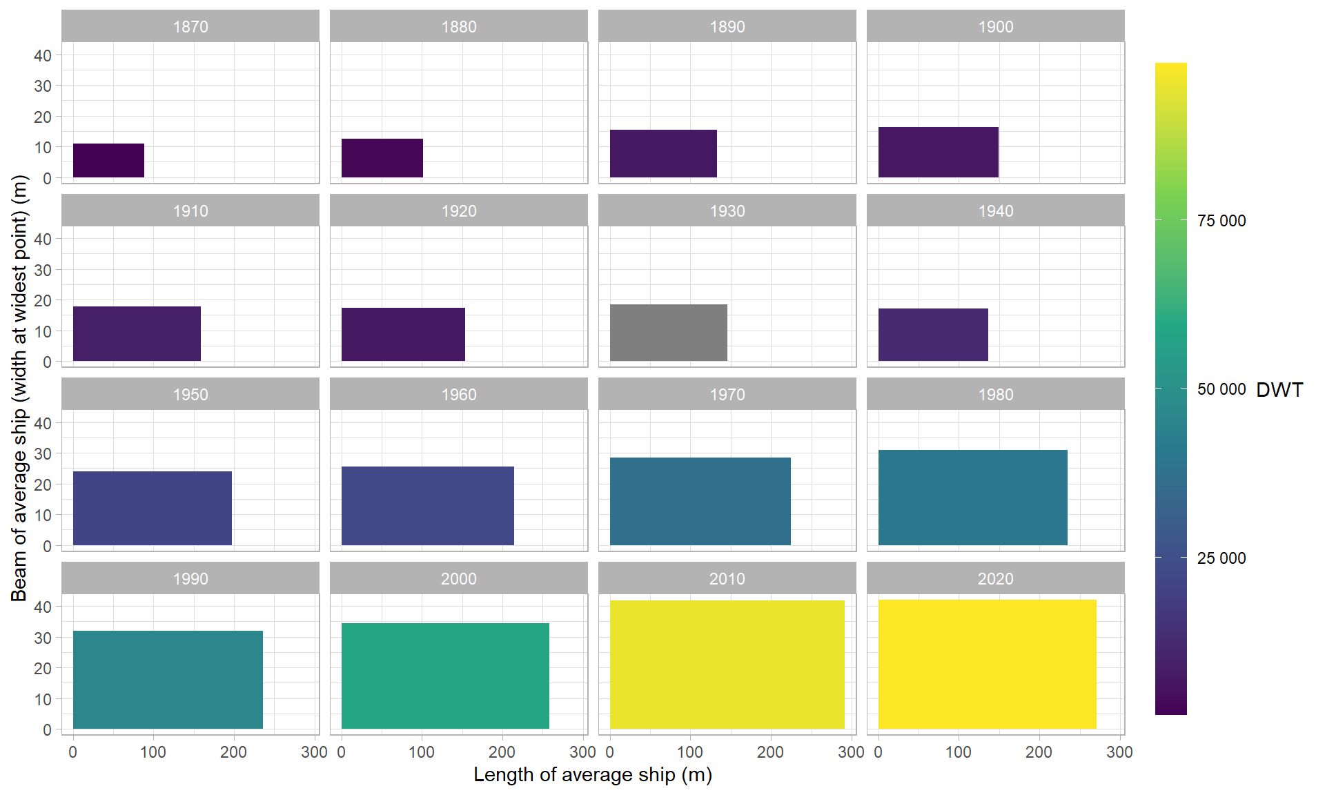
Cargo ships have increased dramatically in size over time! The oldest ship in our dataset is the R. J. Hackett, one of the first Great Lakes freighters. It was just 63m long and 10m wide, with a wooden hull. According to historian Mark Thompson, the R. J. Hackett’s boxy hull, hatch-lined deck, and placement of the deckhouses meant the ship was ideally suited for moving cargo through inland waterways. This steamer greatly influenced the development of cargo ships which followed.
Today, container ships like the Ever Given are nearly 400m long, 60m wide, and can carry more than 20,000 twenty-foot containers. That’s enough space for 745 million bananas!
TEUs, or twenty-foot equivalent units, is the measure that shipping companies use to compare volume. A TEU is 6.1m long, 2.4m wide and usually 2.6m high. Source: Wikipedia
Increasing size of container ships by length, width and tonnage.
In the plots below we focus only on container ships built after 1970. This era saw the construction of the first ships purpose built to carry ISO containers, which could be loaded and unloaded rapidly at port, repacked and shipped onward on any compatible ship, truck or train. The ISO standard container transformed the shipping industry and replaced the prior status quo of break bulk carriers. One of the consequences was a dramatic reduction in demand for “stevedores” or “longshoremen”; workers who would manually unload cargo from break bulk carriers.
If you’re interested in containerization, I highly reccomend this episode from the podcast Trade Talks, and this eight-part series from Alexis Madrigal.
Tonnage over time
How have cargo ship deadweight tonnages, or how much cargo a ship can carry, changed over time? Mouse over a point to see the name of the ship.
Container ships can carry more cargo today than ever before. It’s hard to get my mind around 220 000 tons of cargo!
Length over time
How has the length of cargo ships changed over time? Mouse over a point to see the name of the ship.
The Ever Given is among the longest container ships operating today at 400m in length. The linear fit line shows that there has been a steady increase in container ship length over time.
Width over time
How have cargo ship beams, or widths of ships at their widest point, changed over time? Mouse over a point to see the name of the ship.
Container ships have also become wider, with lumping at beams of 32m, 40m and 59m.
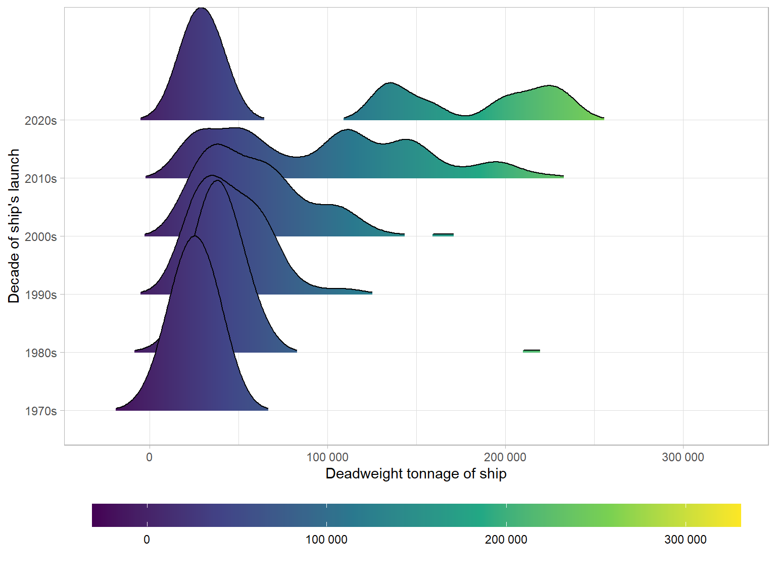
Birfucation in cargo ship capacity.
So it certainly seems that cargo ships have been becoming larger over time. Interestingly, it appears that while the largest container ships continue to get larger and carry more cargo, there is still a need for relatively small ships. There are a significant number of container ships that can carry less than 50 000 tons launched since 2010, shown in the density plot below. We could say that there has been a bifurcation in ship capacity, with a few enormous ships, and a greater number of smaller ships operating in tandem today.
Why have container ships become so large?
Economies of scale describes a decrease in the per unit cost as scale of an operation increases. This perfectly fits the shipping industry’s relentless path towards upsizing ships, cranes and ports. One of the reasons has to do with fluid dynamics. Hull resistance is one of the key factors impacting fuel consumption. For vessels in water, drag loss is less than proportional to increasing cargo carried. In other words, making a ship larger usually results in less fuel consumption per ton of cargo, holding all else constant. As we have seen in the figures above, container ships have become larger and larger as they carry more cargo per ship, in an effort to save fuel.
Other methods of drag reduction include improved hull design, injecting air around the hull surface and reducing hull roughness from slime and weeds. See Resistence and powering of ships 
According to Marc Levinson, author of The Box: How the Shipping Container Made the World Smaller and the World Economy Bigger, the shippers applied this idea to every element of the industry. He says:
Bigger ships lowered the cost of carrying each container. Bigger ports with bigger cranes lowered the cost of handling each ship. Bigger containers — the 20-foot box, shippers’ favorite in the early 1970s, was yielding to the 40-footer — cut down on crane movements and reduced the time needed to turn a vessel around in port, making more efficient use of capital. A virtuous circle had developed: lower costs per container permitted lower rates, which drew more freight, which supported yet more investments in order to lower unit costs even more. If ever there was a business in which economies of scale mattered, container shipping was it.
The consequences of containerization are fascinating – including rapidly falling costs of trade, increasingly intermeshed global supply chains, a proliferation of robots at ports, and the environmental challenges associated with ships, trucks and trains meeting at transshipping nodes around the world.
In the remainder of this post I walk through scraping some of the data presented above.
Scraping Wikipedia’s list of cargo ships.
Now that we have had a look at the data, I want to walk through how it can easily be collected and processed for visualizing with R.
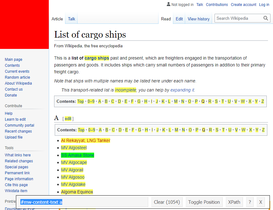
The source of the pre-1970 data is Wikipedia’s list of cargo ships, a screenshot of which I include below. The plan to get the data involves collecting a list of links to each page and then scraping the information about each ship from it’s page. The code chunks below show the process of scraping the data and you can access the scripts on my GitHub repository.
If you want to follow along with a video of the scraping process, I highly recommend this video on ramen reviews from David Robinson.

Screenshot of the list
The list contains the names of the cargo ships in alphabetical order. We want to grab the links to each article from the list. We can use the SelectorGadget tool to highlight the CSS that leads to each ship’s page. SelectorGadget is an open source tool that makes CSS selector generation and discovery on complicated sites a breeze. It allows you to point to a web page element with the mouse and find the CSS selector for that element. It highlights everything matched by the selector.
I show here a picture of the interface with Google’s Chrome browser:
Screenshot showing SelectorGadget interface
Once we have the path we want to collect the links from, we can use the rvest package to scrape the data. Written by Hadley Wickham, this is a package that makes it easy to scrape data from HTML web pages.
We start with the url of the list:
link <- "https://en.wikipedia.org/wiki/List_of_cargo_ships"Function to grab the page link from the list of cargo ships.
Next we write a function that gets the list of links from the page. We begin by reading the HTML from the link, then selecting the nodes with the links, and then the attribute called “href” – the url of the page for each ship. We format the output as a tibble, a data frame object that is convenient to work with. Notably this function will work for any list of pages on Wikipedia, neat!
# function that gets the urls for each page from the list
get_ship_links <- function(link){

  html <- read_html(link)

  # nice little message
  message(glue("Getting links from {link}"))

  html %>%
    # this html node is found with the selector gadget tool.
    html_nodes("#mw-content-text li a") %>%
    # gets the links or href
    html_attr("href") %>%
    # stores them as a tibble, very convenient alternative to a dataframe.
    as_tibble()

}
Here we apply the function to our link and get back a list of links to each page.
# apply function to link.
list_of_links <- get_ship_links(link)
Getting links from https://en.wikipedia.org/wiki/List_of_cargo_shipslist_of_links# A tibble: 8 × 1
value
<chr>
1 /wiki/List_of_Panama-flagged_cargo_ships
2 /wiki/List_of_Liberia-flagged_cargo_ships
3 /wiki/List_of_Malta-flagged_cargo_ships
4 /wiki/List_of_Russia-flagged_cargo_ships
5 /wiki/List_of_Bangladesh-flagged_cargo_ships
6 /wiki/List_of_Greece-flagged_cargo_ships
7 /wiki/List_of_bulk_carriers
8 /wiki/List_of_cruise_ships We can see we get 1 024 links back, but the problem is that there are multiple instances of the Table of Contents links, “#A”, “#B” etc. We will filter these out by only selecting links with 5 or more characters.
list_of_links <- list_of_links %>%
  filter(nchar(value) > 4) %>%
  # this sticks the stub to the link so that we can use it later
  mutate(value = str_c("https://en.wikipedia.org/", value)) %>%
  select(url = value)

list_of_links
# A tibble: 8 × 1
url
<chr>
1 https://en.wikipedia.org//wiki/List_of_Panama-flagged_cargo_ships
2 https://en.wikipedia.org//wiki/List_of_Liberia-flagged_cargo_ships
3 https://en.wikipedia.org//wiki/List_of_Malta-flagged_cargo_ships
4 https://en.wikipedia.org//wiki/List_of_Russia-flagged_cargo_ships
5 https://en.wikipedia.org//wiki/List_of_Bangladesh-flagged_cargo_ships
6 https://en.wikipedia.org//wiki/List_of_Greece-flagged_cargo_ships
7 https://en.wikipedia.org//wiki/List_of_bulk_carriers
8 https://en.wikipedia.org//wiki/List_of_cruise_ships Now that we have the list of links we can get the data about each ship from its Wikipedia page. We want it’s date of launch, it’s type, tonnage, length, beam and status (in service, retired, destroyed etc.). This is all stored helpfully in the infobox on each page:

Screenshot showing page for ship called Algosteel
SelectorGadget helps us out again, returning a path to the infobox:
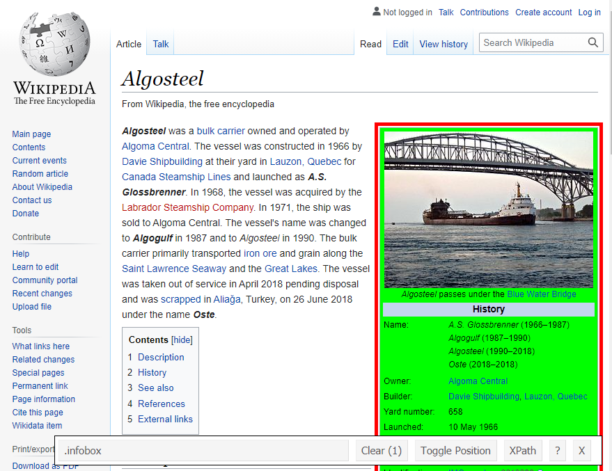
Screenshot the infobox selection for the Algosteel
Function to scrape the information about each ship.
Here is little function that returns infobox from page about the Algosteel. It has a nice helper message to tell us that it is working, grabs the tabular information, and returns it as a tibble.
url <- "https://en.wikipedia.org/wiki/Algosteel"

get_ship_info_wiki_list <- function(url){
  # store the html from the page
  html <- read_html(url)
  # nice message so that we can see progress.
  message(glue("Getting info from {url}"))

  data <- html %>%
    html_node(".infobox") %>%
    html_table() %>%
    rename(title = X1,
           value = X2)

  data

}
Here is the output we get back from the Algosteel.
get_ship_info_wiki_list(url)Getting info from https://en.wikipedia.org/wiki/Algosteel# A tibble: 18 × 2
title value
<chr> <chr>
1 Algosteel passes under the Blue Water Bridge "Algosteel passes under the Blu…
2 History "History"
3 Name "A.S. Glossbrenner (1966–1987)\…
4 Owner "Algoma Central"
5 Builder "Davie Shipbuilding, Lauzon, Qu…
6 Yard number "658"
7 Launched "10 May 1966"
8 Completed "July 1966"
9 Out of service "April 2018"
10 Identification "IMO number: 6613299"
11 Fate "Scrapped 2018"
12 General characteristics "General characteristics"
13 Type "Bulk carrier"
14 Tonnage "17,955 GRT\n26,690 DWT"
15 Length "222.4 m (729.7 ft) oa\n216.2 m…
16 Beam "23.0 m (75.5 ft)"
17 Installed power "1 × shaft, diesel engine"
18 Speed "14.5 knots (26.9 km/h; 16.7 mp…We do not care about all of this information, so we will filter for what we want to retain later.
Scraping each page
The code below iterates through the list of links and returns the information in the infobox from each page. The possibly statement is a helpful function from the purrr package that allows us to return a message if the operation fails, in this case a string that just says “failed”.
For more about the usefulness of
purrr’s safely functions see Dealing with failure in R for Data Science by Hadley Wickham and Garrett Grolemund.# mapping through each url
df <- list_of_links %>%
# the possibly statement here means that we will record if there is a failure, for example if there is no infobox in an article.
mutate(text = map(url, possibly(get_ship_info_wiki_list, "failed")))We get back a tibble with a nested column that contains the information scraped from each page. We remove the ships that failed (the ones that succeeded will have an NA in the text field, while the ones that failed will say “failed”).
df <- df %>%
  unnest(text) %>%
  filter(is.na(text)) %>%
  select(-text)
Next we select the information from the infobox that we want to keep; name, launch date, status, tonnage, length and width.
df <- df %>%
  mutate(value = str_squish(value)) %>%
  group_by(url) %>%
  mutate(row_id = row_number()) %>%
  filter(title %in% c("Name:",
           "Launched:",
           "Status:",
           "Tonnage:",
           "Length:",
           "Beam:")) %>%
  # then we pivot wider so that each ship is one row
  pivot_wider(names_from = title, values_from = value) %>%
  # cleaning the names makes it easier to use these columns later
  janitor::clean_names() %>%
  ungroup() %>%
  select(-row_id) %>%
  group_by(url) %>%
  # removing the superfluous columns
  summarise_all(funs(na.omit(.)[1]))

write_rds(df, "data/cargo_ship_info.rds")
Here is the output! Easy as that. We can put it in a nice table and then hyperlink the article in the url column.
Thanks for reading along, and I hope that you come back for the next article in the series.
Part 2 will look at unsupervised machine learning methods.
Footnotes
I focus on all cargo ships until the 1970s, whereafter I focus only on container ships. Additional data on container ships is scraped from VesselFinder.com↩︎